Diffusion Models
Part A: Exploring the Power of Diffusion!
A.0: Trying it Out
I ended up using seed=28 over the course of this project.
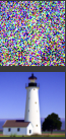
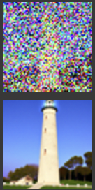
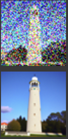
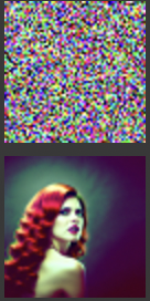
The following are two sets of images produced by DeepFloyd's image diffusion model! The descriptors on which the images were conditioned as well as the number of inference steps I had the model execute are both given.
DeepFloyd Generated Images
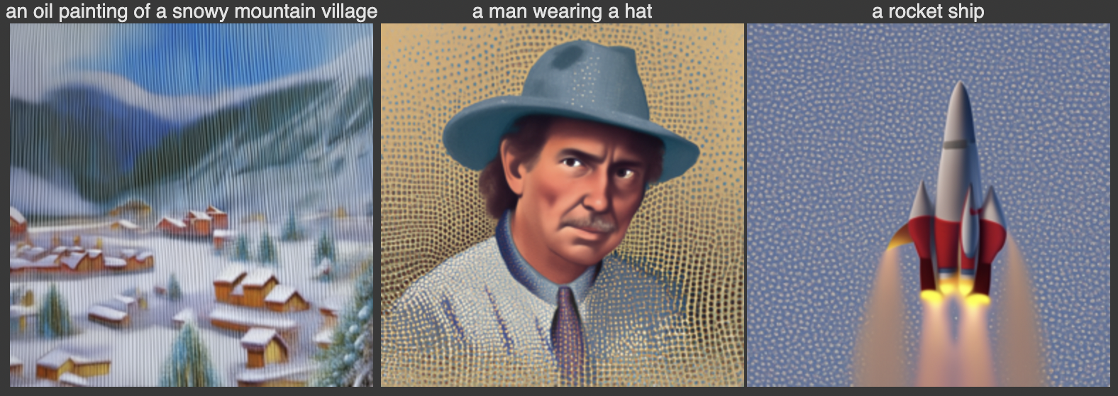
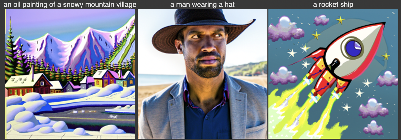
Notably, increasing the number of inference steps improved the quality, specificity, and image-to-noise ratio.
A.1: Sampling Loops
1) Forward Process Implementation (Noising)
The first thing I did is experiment with nosing the following are my base image (only 64x64 for runtime purposes), and noised images at varying noise levels.
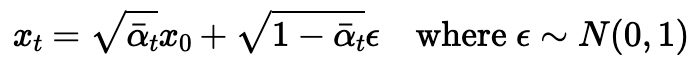
Formula used for noising
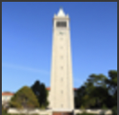
Base Image
Noised Base Image
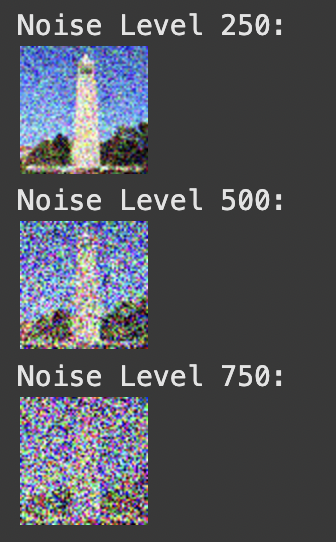
The various noise levels represent indices of "alpha_cumprod", the cummulative product of alphas used to transition an image from clean to noisy.
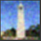
1.2) Classical/Gaussian Denoising
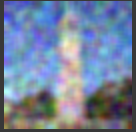
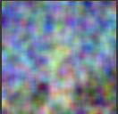
The naive approach to denoising is Gaussian blur filtering. The results of denoising from each of the above noise levels via this method is shown below.
Noise Level 250
Noise Level 500
Noise Level 750
1.3) One-Step Denoising
In this section, the denoising process is performed using a UNet model. The steps include:
- Estimating noise in the noisy image using
stage_1.unet. - Removing the estimated noise to recover an approximation of the original image.
Noise Level 250
Below are the results for noise level 250:
Noise Level 500
Below are the results for noise level 500:
Noise Level 750
Below are the results for noise level 750:
1.4) Iterative Denoising
In this section, iterative denoising is applied. The images were first noised to a high level (t = 750) and then iteratively denoised at decreasing noise levels. This process demonstrates the improvement at various stages of denoising, showing how the model progressively reconstructs the original image.
Iterative Denoising Steps
Comparison of Final Results
Comparing the results of iterative denoising, Gaussian denoising, and one-step denoising reveals key differences:
- Gaussian Denoising: This method blurred the existing noise, resulting in a degraded image quality. It failed to remove noise effectively and, in many cases, worsened the appearance of the image.
- One-Step Denoising: While this approach reduced noise significantly, the final result was overly blurry, lacking finer details and clarity. It produced a passable result but could not fully restore the image.
- Iterative Denoising: This approach consistently outperformed the others by iteratively removing noise and reconstructing the image. The model went beyond simply removing noise—it creatively reconstructed details to produce a high-quality image that closely resembled the original.
Iterative denoising demonstrates the model's ability to "hallucinate" and reconstruct fine details by leveraging multiple steps, making it the most effective approach in this comparison.
1.5) Diffusion Model Sampling
In this section, the diffusion model is used to generate images from scratch. By setting i_start = 0 and passing in pure random noise, the model iteratively denoises the noise to generate a high-quality image. Below are five sampled results:
Generated Images
1.6) Classifier-Free Guidance (CFG)
In the previous section, the generated images were often of poor quality, and some were nonsensical. To address this, we employ Classifier-Free Guidance (CFG), a technique that can significantly improve image quality at the cost of some image diversity.
CFG works by combining a conditional and an unconditional noise estimate. The new noise estimate is computed as:
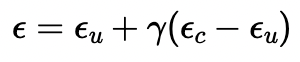
The parameter γ determines the strength of CFG. For γ = 0, the result is an unconditional noise estimate. For γ = 1, the result is a conditional noise estimate.
When γ > 1, the model amplifies the differences between these two estimates, often leading to much higher quality images.
To implement this, I modified the iterative_denoise function to include CFG, using a CFG scale of γ = 7.
I used the prompt "a high quality photo" to guide the diffusion model and generated the following results:
Generated Images with Classifier-Free Guidance


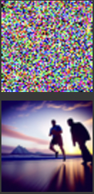
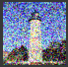
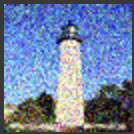
1.7) Image-to-image Translation
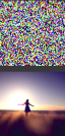
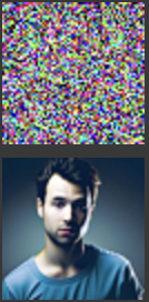
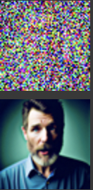
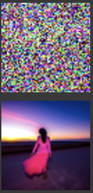
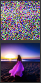
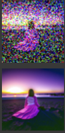
In this section, I used the diffusion model with Classifier-Free Guidance (CFG) to perform image-to-image translation. Starting from a test image, noise was added at different levels, and the iterative denoising process gradually restored the image while conditioning on the prompt "a high quality photo". Both the noised and denoised versions of each image are displayed together in a single combined image for better comparison.
Test Image 1: Gradual Denoising
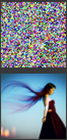
Test Image 2: Gradual Denoising

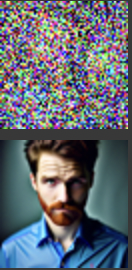

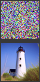
Test Image 3: Gradual Denoising


1.7.1) Editing Hand-Drawn and Web Images
In this section, I experimented with applying edits to non-realistic images, such as hand-drawn sketches and web images, using the iterative denoising process with Classifier-Free Guidance (CFG).
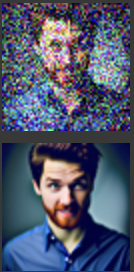
Starting from the noisy versions, the images were progressively denoised at different levels of noise (i_start = 1, 3, 5, 7, 10, 20).
Note that a higher i_start value corresponds to a lower noise level or a later time step in the denoising process, leading to outputs that are closer to the original image.
Web Image: Gradual Denoising


Hand-Drawn Image 1: Gradual Denoising


Hand-Drawn Image 2: Gradual Denoising


Two key observations:
- Noising the image too much prior to diffusion results in a completely new image.
- Not noising the image enough yields (close to) the original image.
When the image is noised just right, the model has just enough structure to produce what was requested, but not enough to produce the same as what was requested. Therefore, it fills in the gaps with the image data its been trained on, producing a "realistic" version of the original image!
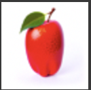
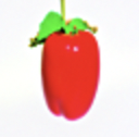
1.7.2) Inpainting
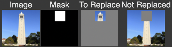
In this section, I applied inpainting to modify specific parts of an image while preserving other regions. Using a binary mask, areas with a value of 0 remain unchanged, while areas with a value of 1 are edited through the iterative diffusion process. This allows new content to be generated in selected regions, following the methodology described in the RePaint paper.
Setup
Inpainting Process
The inpainting process progressively restores the masked area using decreasing noise levels. Below are the intermediate steps and the final result:
The inpainting process shows how the masked area is gradually modified through successive iterations, leading to a realistic reconstruction that blends seamlessly with the unaltered parts of the image.
1.7.3: Text-Conditional Image-to-image Translation
In this section, I used the same process as SDEdit but added a text prompt to guide the projection.
Instead of only projecting to the natural image manifold, the model incorporates a textual description to further influence the output.
This process modifies the image to align both with the original content and the prompt.
Below are the results for three test images, progressively denoised at different noise levels (t = 960, 900, 840, 780, 690, 390).
Note: Each image combines both the noised and denoised versions for easier comparison.
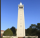
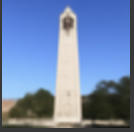
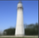
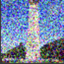
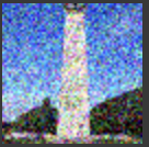
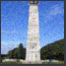
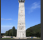
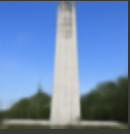
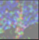
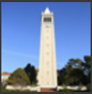
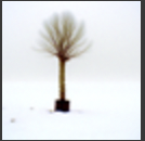
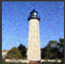
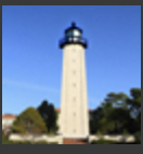
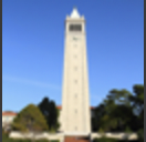
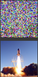
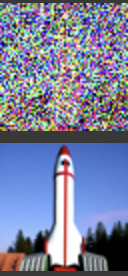
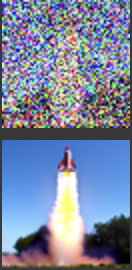
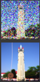
Test Image 1: Campanile with the Prompt "a rocket ship"
This test starts with an image of the Campanile and applies the text prompt "a rocket ship". The model transforms the image to incorporate elements of a rocket ship while gradually removing noise.


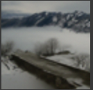
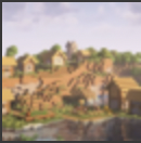
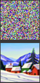
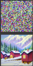
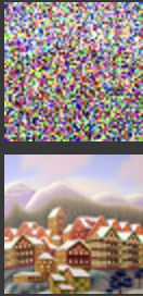
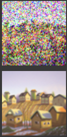
Test Image 2: Minecraft Village with the Prompt "an oil painting of a snowy mountain village"
This test starts with an image of a Minecraft village and applies the text prompt "an oil painting of a snowy mountain village". The model transforms the blocky landscape into a more painterly and snowy aesthetic while gradually removing noise.


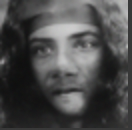
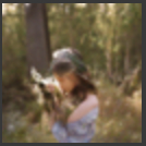
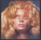
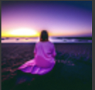
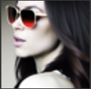
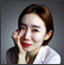
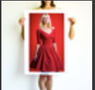
Test Image 3: Woman Wearing a Hat with the Prompt "a man wearing a hat"
This test starts with an image of a woman wearing a hat and applies the text prompt "a man wearing a hat". The model adjusts the facial features and appearance to align with the prompt while preserving the overall hat element.
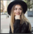
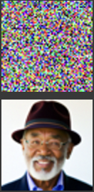
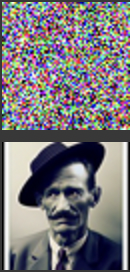
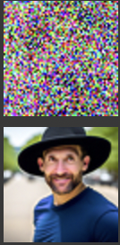

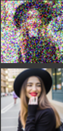
Interestingly, the final results appear to have a hybrid quality, combining elements of the original image and the influence of the text prompt, with the last images being the best blend for the campinile x rocket and mc village x snowy village, and the second last image being best for the woman x man blend. This behavior closely resembles what I aim to achieve explicitly in Section 1.9, where the model generates hybrid images directly from scratch using specific textual guidance.
1.8: Visual Anagrams
In this section, I implemented visual anagrams using the diffusion model. By averaging the noise estimates for two different prompts and orientations (right-side-up and upside-down), the model generates images that look different depending on how they are viewed.
Below are the results for three visual anagrams, each generated with two prompts. The same image is displayed twice: once upright and once flipped upside-down to highlight the illusion.
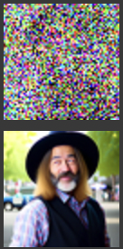
Image 1
Prompts: "an oil painting of people around a campfire" (right-side-up) and "an oil painting of an old man" (upside-down).
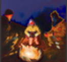
Image 2
Prompts: "a photo of a hipster barista" (right-side-up) and "a rocket ship" (upside-down).

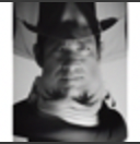
Image 3
Prompts: "a man wearing a hat" (right-side-up) and "a photo of a man" (upside-down).
1.9: Hybrid Images
In this section, I implemented hybrid image generation using the Factorized Diffusion technique. By combining low-frequency components from one noise estimate with high-frequency components from another, the model creates images that appear different depending on the viewing distance.
The total noise used in generating the hybrid images is calculated using the following equation:
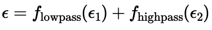
This equation shows how the low-frequency and high-frequency noise components are combined to form the total noise, allowing the model to blend two prompts effectively.
Below are the results for three hybrid images, each generated with two prompts.
Image 1: Skull and Waterfalls
Prompts: "a lithograph of a skull" (low frequencies) and "a lithograph of waterfalls" (high frequencies).
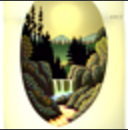
Image 2: Old Man and People Around a Campfire
Prompts: "an oil painting of an old man" (low frequencies) and "an oil painting of people around a campfire" (high frequencies).
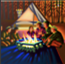
Image 3: Rocket Ship and Pencil
Prompts: "a rocket ship" (low frequencies) and "a pencil" (high frequencies).

Similar to project 2, the low-pass filtered images are visible from a distance, the high-pass filtered images are more obvious from up close. Our AI seamlessly integrates the two!
Part B: Exploring the Power of Diffusion!
This part of the project was extremely interesting and ultimately rewarding! I got to write and train my own diffusion model on MNIST digit images.
B.1: Training a Single-Step Denoiser UNET
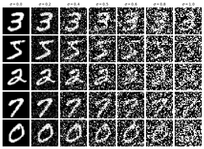
B.1.1: Visualizing the Noising Process
To begin, we visualized the noising process by applying Gaussian noise to the MNIST dataset at varying levels of σ.
This process demonstrates how images are progressively corrupted as the noise level increases.
The visualization below shows the results for σ values ranging from 0.0 (no noise) to 1.0 (maximum noise):
B.1.2: Training the Single-Step Denoiser
The UNet model was trained to denoise images at a fixed noise level of σ = 0.5.
This approach, referred to as "single-step diffusion," does not involve iterative refinement. Instead, the model directly learns to map a noised image to its corresponding clean version in a single step.
During training, the Mean Squared Error (MSE) loss was minimized between the model’s prediction and the original (clean) image. This method is computationally efficient, as the model only needs to handle a single noise level, but it limits its generalizability to unseen noise distributions.
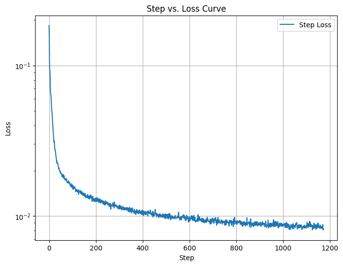
The graph above shows the training loss decreasing steadily over iterations.
This indicates that the model is successfully learning to denoise images at σ = 0.5, reducing the error between its predictions and the original images.
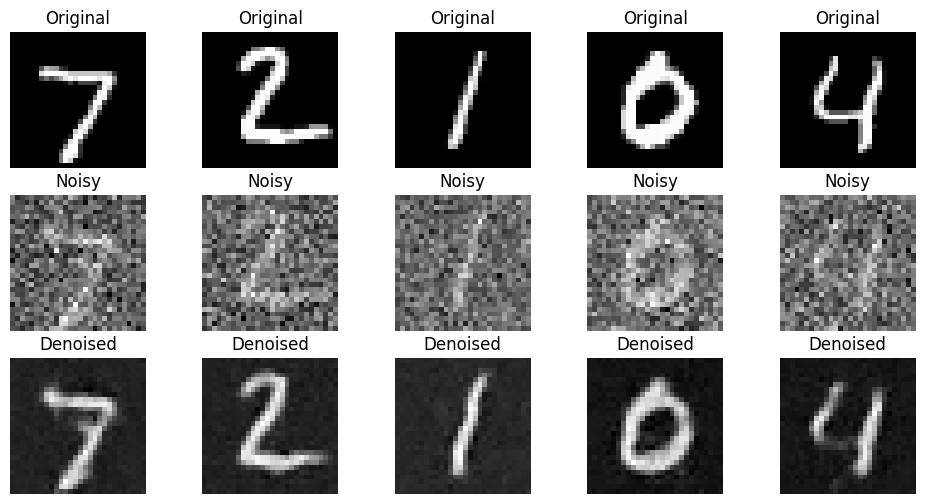
After the first epoch, the model begins to produce results that are recognizable but still noisy. This early stage demonstrates the initial progress made by the model as it starts to understand the mapping from noisy to clean images.
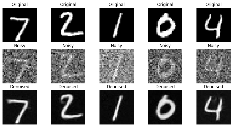
By the fifth epoch, the model produces significantly improved outputs. The reconstructed images closely resemble the original clean images,
indicating that the single-step denoiser has effectively learned to handle noise at σ = 0.5.
B.1.3: Testing on Out-of-Distribution Noise Levels
Finally, we evaluated the model on images noised at different levels of σ, ranging from 0.0 to 1.0.
This is referred to as out-of-distribution testing because the model was only trained at σ = 0.5.
The results highlight the limitations of the single-step approach, as the model struggles to generalize to noise levels outside its training distribution.
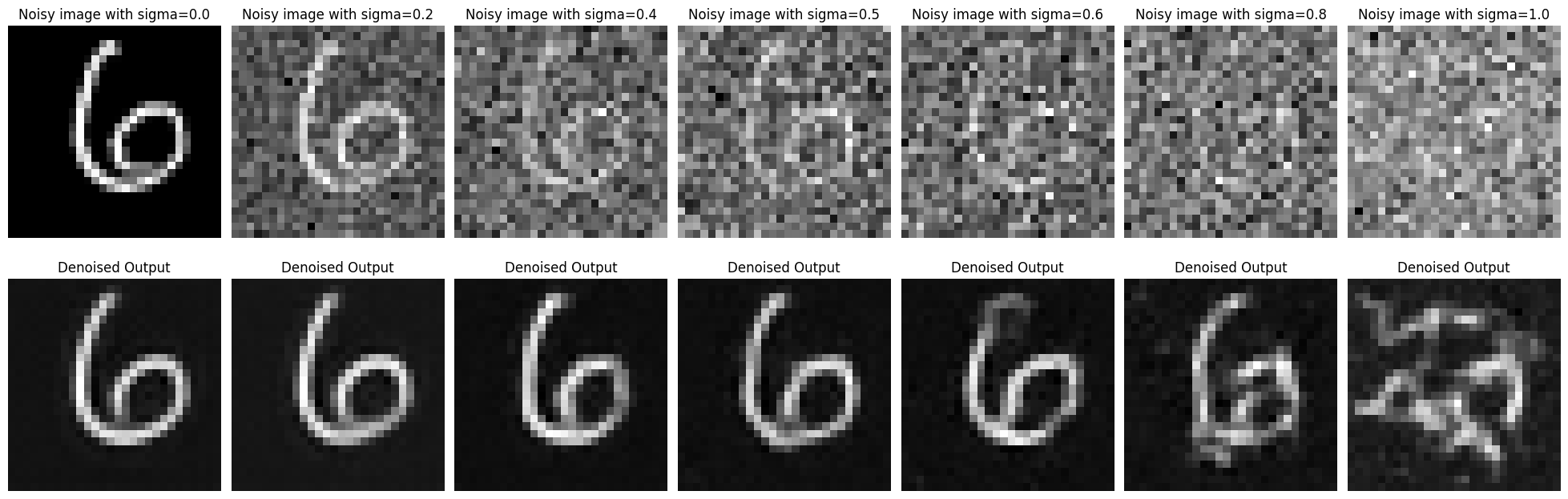
While the model performs well at σ = 0.5, its ability to denoise images deteriorates at higher noise levels.
This highlights a key limitation of single-step denoising and motivates the exploration of multi-step approaches in future work.
In summary, this section demonstrated the training and evaluation of a single-step denoiser. While effective for its intended noise level, this method is constrained in its generalizability, prompting further exploration of iterative denoising techniques.
B.2: Training a Diffusion Model
This was the most fascinating portion of the project for me! In it, I had the opportunity to code diffusion from scratch! Noisy images were transformed to MNIST digits
Part 1:
In this section, we extend the single-step denoising UNet by introducing time-conditioning. The model is now trained to denoise images at various noise levels by using a time-conditioning parameter. This modification enables the UNet to generalize across multiple noise levels rather than being restricted to a single fixed noise level like before.
However, the MNIST digit labels themselves are not used in this model. As a result, while the denoised images are clean digits, they lack specificity or clarity since the model is not conditioned on any class-based information. This lack of conditioning leads to results that are somewhat blurry, similar to the issues observed in Part A of this project, where insufficient conditioning limited the sharpness of the generated outputs.
Training Process
During training, the UNet was exposed to images corrupted at various noise levels and was tasked with reconstructing the original images. Below are the key results from this process:
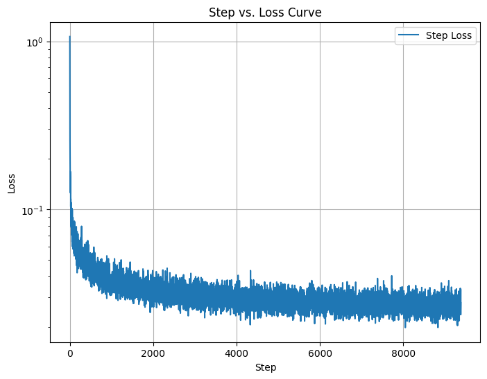
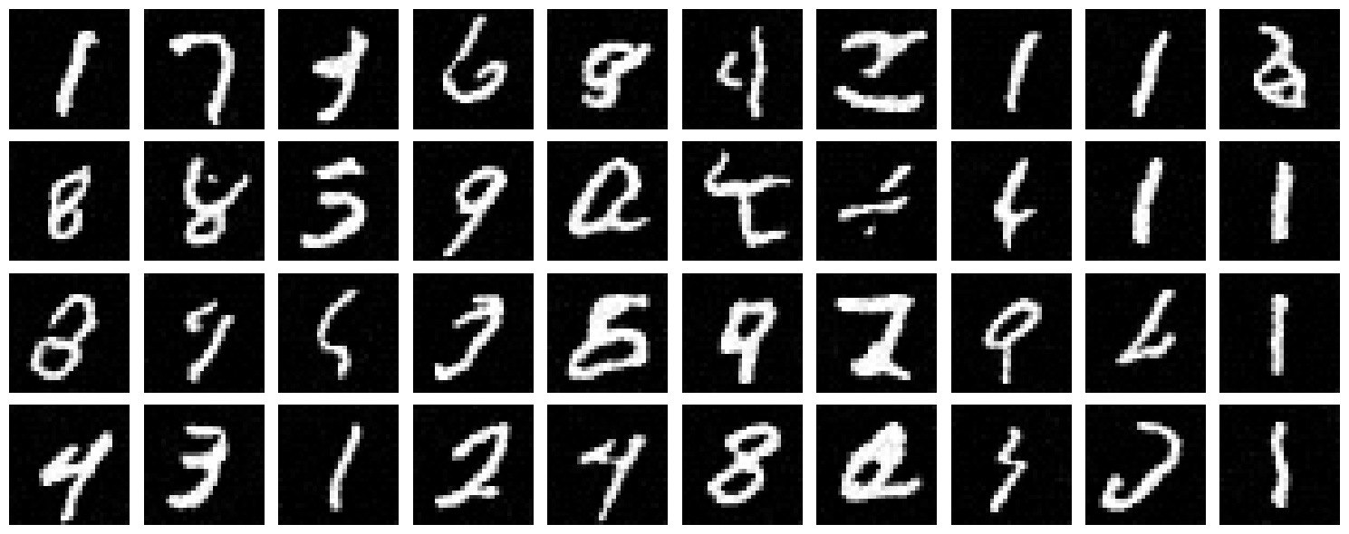
As seen from the results, the training loss decreases steadily, indicating the model is learning to reconstruct clean images from noisy inputs. However, the lack of digit label information in this implementation means the outputs are clean but not sharply defined. This reinforces the importance of conditioning the model on additional context to improve its generative capabilities.
In the next part, we will introduce class-conditioning, which is expected to significantly improve the results by incorporating label-based guidance to refine the outputs further.
Part 2:
To address the limitations observed in the time-conditioned model, we introduced class conditioning in this section. By utilizing the labels of the MNIST dataset, the model is now trained to not only denoise the images but also to produce specific digit classes. Class conditioning allows the model to utilize label information effectively, leading to sharper and more coherent outputs compared to the unconditioned model.
Class conditioning was incorporated into the UNet architecture by adding two additional fully connected blocks (FCBlocks) to process the class-conditioning vector c. This vector is encoded as a one-hot representation of the digit labels (0-9). To ensure the model can still handle unconditioned scenarios, we applied dropout, where the class-conditioning vector is set to zero 10% of the time (p_uncond = 0.1).
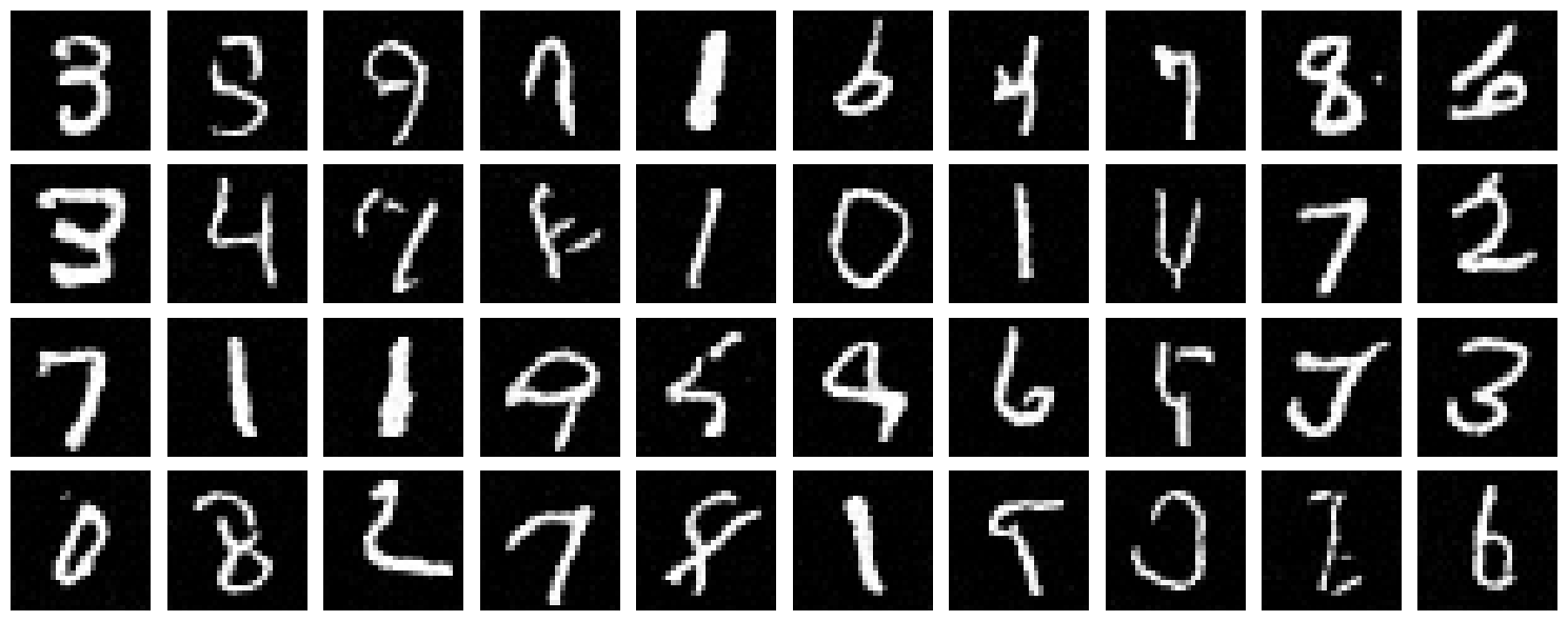
The final model is conditioned on both the time step t and the class c, enabling it to reconstruct images at specific noise levels while also generating digits corresponding to the provided class label. This enabled us to generate from an arbitray noise level (and in particular, iteratively from pure noise) a handwritten digit of optionally specified class.
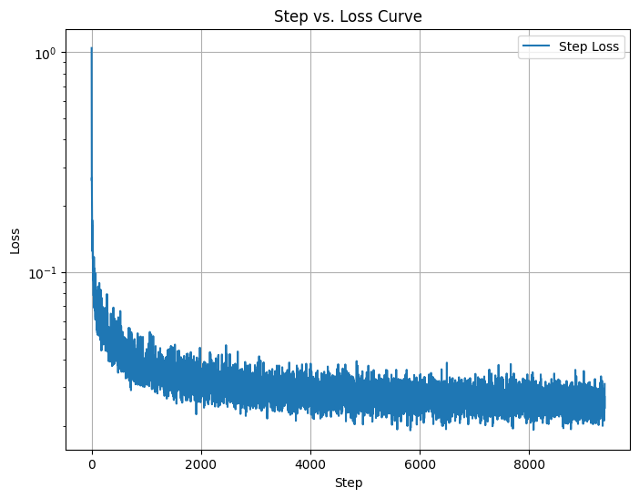
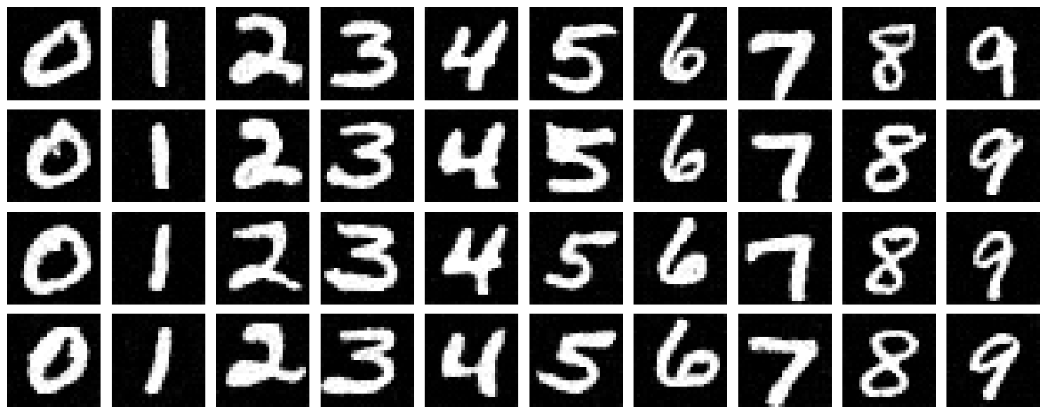
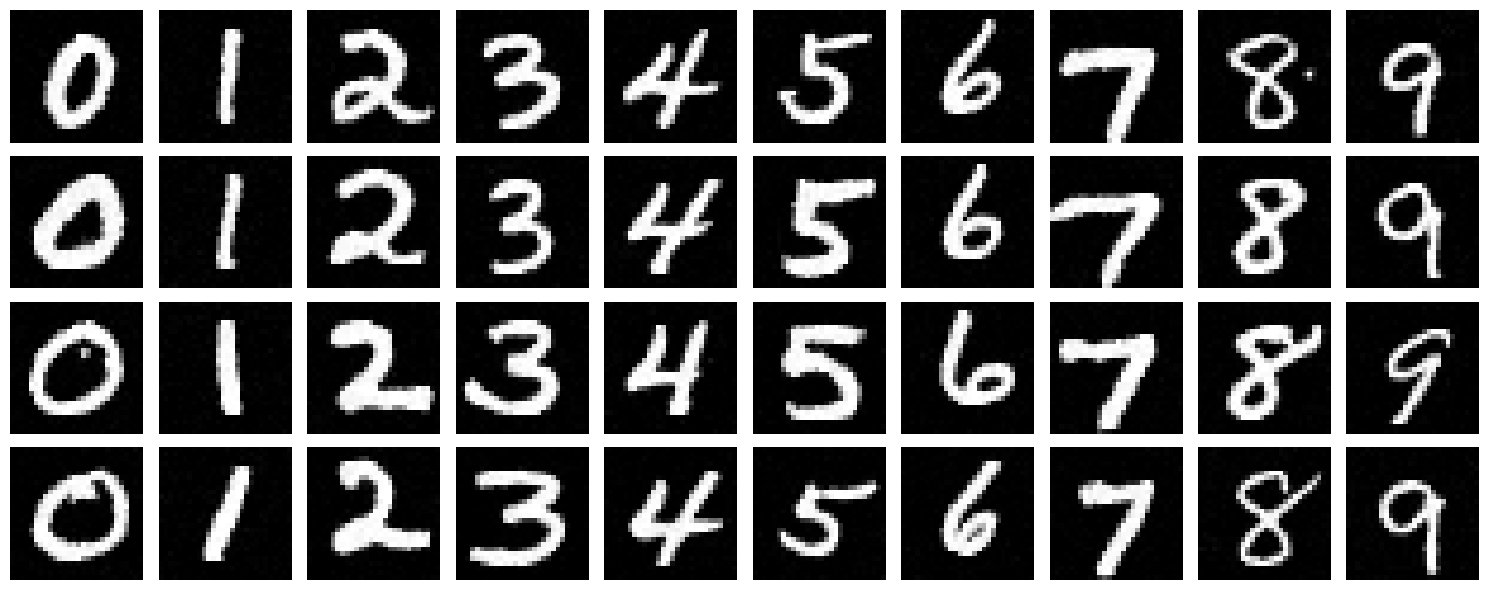
The training loss curve shows a steady decrease, indicating the model effectively learns to denoise and reconstruct specific digit classes from noisy inputs. The results after 5 and 20 epochs demonstrate a significant improvement in the sharpness and clarity of the generated digits compared to the unconditioned model. By explicitly conditioning on both time and class, the outputs become not only clean but also class-specific, addressing the limitations observed in the earlier implementations.
Conclusion
This project provided a comprehensive exploration of diffusion models, I really enjoyed it!